Statistical Analysis of MRI Data

Author: Syeda Warda Taqdees

Contributor/s: Dr. Christina Tuke Flanders

Learning Objectives

After completing this lesson, students should be able to

• Normalize MRI data for implementing image processing methods.
• Create color-coded masks for image regions.
• Calculate statistical parameters such as mean voxel values of image regions.
• Display histograms of image regions for quantitative ROI analysis.
• Calculate and display empirical probability distributions of image regions.

We can detect pathology in MRI image by calculating statistical properties of abnormal tissue and comparing them with the properties of a healthy tissue sample.

Color-Coding ROIs

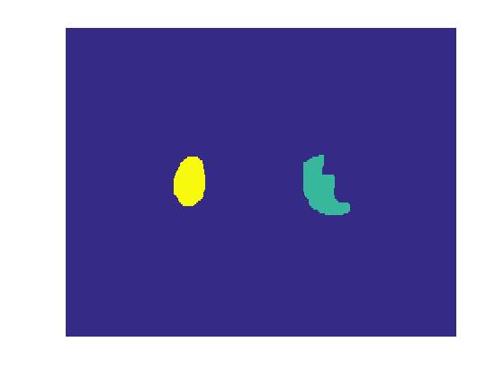
First, we select two ROIs in slice#15 of the given dataset using imfreehand(). Voxels from each regions are assigned a unique number, starting from 1, in image mask. We can later use the color-coded mask image to label ROIs.

% Selecting ROI for analysis
figure
imagesc(mriImage1)

for iReg = 1:2
     hFree= imfreehand();
     regionBW(:,:,iReg) = createMask(hFree);
     codedRegionBW(:,:,iReg) = iReg.*regionBW(:,:,iReg);
     [regX regY regVox(iReg).Vals] = find(regionBW(:,:,iReg) .* mriImage1);
     delete(hFree);
end

Let's display the color-coded mask. The green region 'R1' on the right is the pathology and the yellow region 'R2' on left is normal tissue.

% Creating region-coded mask
codedRegionMask = sum(codedRegionBW,3);

% Displaying region-coded mask
figure
imagesc(codedRegionMask);
axis off;

Image Statistical Parameters

After selecting normal and tumor ROIs, lets calculate mean and std of T2 values in both regions.

% Display mean voxel values of both ROIs
disp(sprintf('Mean voxel value of R1: %d',mean(regVox(1).Vals)));
disp(sprintf('Mean voxel value of R2: %d',mean(regVox(2).Vals)));

% Display std. voxel values of both ROIs
disp(sprintf('Standard deviation of R1: %d',std(regVox(1).Vals)));
disp(sprintf('Standard deviation of R2: %d',std(regVox(2).Vals)));

Observe that both mean and std values of tumor region are significantly higher than the normal tissue.

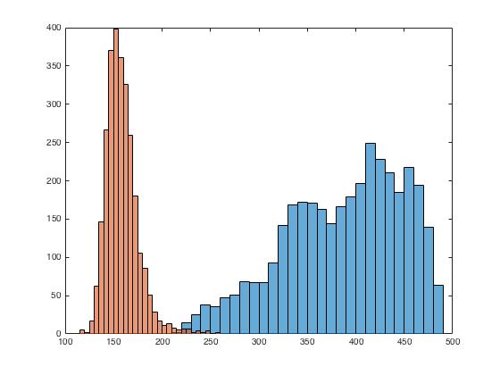
To further investigate the differences in the two image regions, we plot their histograms. The function 'histograms' accepts raw data and plots a histogram with uniform bin width chosen to cover the entire range of value in raw data. The automatic binning algorithm selects an optimal bin width to reveal the underlying data distribution.

% Creating histogram of region voxel values
figure
histogram(regVox(1).Vals)
hold on
histogram(regVox(2).Vals)

Observe that the histograms are separated, indicating towards the changes in the brain tissue due to tumor.

Empirical Probability Distribution

To calculate empirical probability distribution (pdf), we store the histogram information into a 'histogram' object.

% Creating empirical distribution of T2 Values in selected ROIs

% Recalculating histogram and storing the output into a 'Histogram'
% object
hReg1 = histogram(regVox(1).Vals);
hReg2 = histogram(regVox(2).Vals);

The 'histogram' object is a structure that stores all arguments returned by 'histogram' function. These arguements include bin width, number of bins and bin values.

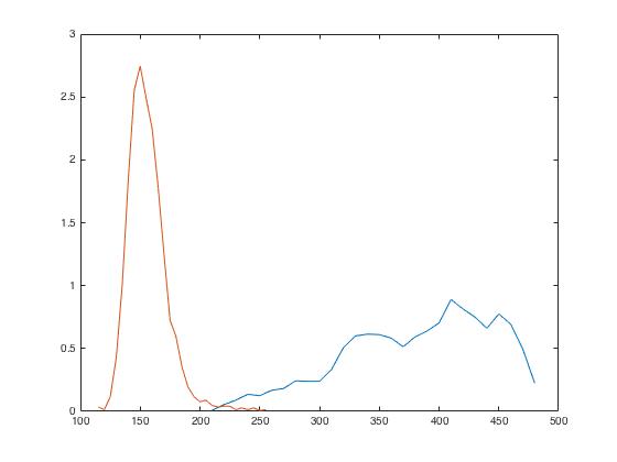
Next, we use the information contained in 'histogram' object to calculate empirical pdfs of R1 and R2.

% Calculating empirical PDFs from above histograms
ePdfReg1 = hReg1.Values./ (hReg1.BinWidth * hReg1.NumBins);
ePdfReg2 = hReg2.Values./ (hReg2.BinWidth * hReg2.NumBins);

We plot both empirical pdfs calculated against each bin edge of the histogram.

% Plotting empirical PDFs
figure;
plot(hReg1.BinEdges(1:end-1), ePdfReg1);
hold on
plot(hReg2.BinEdges(1:end-1), ePdfReg2);

Challenge!

% Challenge 1:
% Take slice# 10 of T2 brain dataset (mriImage1) and select three ROIs -
% Possible abnormality on right, healty tissue on left and right
% ventricle. 
% Find meand and standard deviation of all 3 ROI values
% Plot histogram for each selected ROI and derive empirical probability
% distribution. 
% Try to figure out the nature of pathology based on your observations.
% e.g. Is liquid content present or not etc.