3D Structural Modeling

Author: Rosita Shishegar

Contributor/s: Warda Syeda

Learning Objectives

After finishing this lesson, the students should be able to:

Demonstrate basic knowledge of 3D volumes and surfaces.
Extract the 3D surface of a 3D volume.
Visualise 3D surfaces and color coded surface attributes.
Display 3D anatomical models.
Read and write various 3D surfaces formats in MATLAB.

Anatomical volume is a set of 2D binary masks created from CT or MRI scanner data. The surface model extraction and visualization is commonly used to study the geometry of anatomical structures. In this part, we will study about making 3D volumes and surfaces using MATLAB.

Simulated data

We are going to create simulated cube volume. To make the volume, value 1 is assigned to voxels in the 3D space that belong to inside our geometrical shape.

% Create a 40x40x40 cube in the center of a 140x140x140 frame 
frameDim = 140;       % declaring frame dimensions


% Define cube center aligned to the center of the frame
centerX = frameDim/2;
centerY = frameDim/2;
centerZ = frameDim/2;
xCubeDim = 40;
yCubeDim = 40;
zCubeDim = 40;
 
% Make temperory image array 
tempImage = zeros(frameDim,frameDim,frameDim);
tempImage(centerX-xCubeDim/2:centerX+xCubeDim/2, ...
          centerY-yCubeDim/2:centerY+yCubeDim/2, ...
          centerZ-zCubeDim/2:centerZ+zCubeDim/2 ) = 1;

% Create 3D cube
myCube = tempImage;

% Make a 3D grid
[Y X Z] = meshgrid(1:frameDim,1:frameDim,1:frameDim);  %matlab saves in a different order so X must be Y

The function 'meshgrid' can be used to create a 3D rectangular grid.

To create a surface from the simulated volume data, 'isosurface' is used. This function accepts a 3D volume and returns faces and vertices of the constructed surface in the form of a triangulated mesh.

% Build 3D cube surface
myCubeSurface = isosurface(myCube);

To display the constructed surface, 'patch' function creates and visualizes polygons defined by the faces and vertices of the isosurface (see Fig. 1 & Fig. 2-1).

% Visualise 3D cube surface   % Create polygons for visualising surfaces
figure; 
myCubeHandle = patch(myCubeSurface,'FaceColor','g');   % plotting surface

Certain functions such as 'view', 'camlight' and 'axis' can be used to visually improve the displayed surface.

view([45,20])      % Setting view
camlight(-10,10)   % Adjusting camera light
axis equal         % Sets equal data unit lengths along each axis.
title('Fig.1')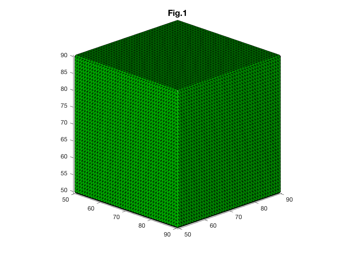

Changing patch properties allows us to control and change appearance and behavior of the 3D surface. For instance, 'FaceColor' sets the color of the polygons. 'Edgecolor' controls the color of polygon edges (Fig. 2-2).

figure
% Plot surface
subplot(2,2,1)
patch(myCubeSurface,'FaceColor','g');   % plotting surface
view([45,20])      % Setting view
camlight(-10,10)   % Adjusting camera light 
axis equal
title('Fig.2-1')

%Plot surface with no edge color
subplot(2,2,2) 
patch(myCubeSurface,'FaceColor','g','EdgeColor','none');
view([45,20])
% camlight with no argument is same as camlight('right') %%%add more explanation
camlight(-10,10)
axis equal
title('Fig.2-2')

Sometimes, one surface could be hidden behind another surface. Setting 'FaceAlpha' property allows us to control the level of transparency of the object thus making it possible to view the hidden details (Fig. 2-3).

% Change surface color and transparency
subplot(2,2,3) 
patch(myCubeSurface,'FaceColor','r','EdgeColor','none','FaceAlpha',0.2);
view([45,20])
camlight(-10,10)
axis equal
title('Fig.2-3')

'patch' also accepts separately specified faces and vertices apart from accepting a whole surface object created by 'isosurface' function (See Fig. 2-4 which presents similar cube as Fig. 2-2).

% Specify surface 'faces' and 'vertices' separately to patch
subplot(2,2,4) 
patch('Faces',myCubeSurface.faces,'Vertices',myCubeSurface.vertices,'FaceColor','r','EdgeColor','none');
view([45,20])
camlight(-10,10)
axis equal
title('Fig.2-4')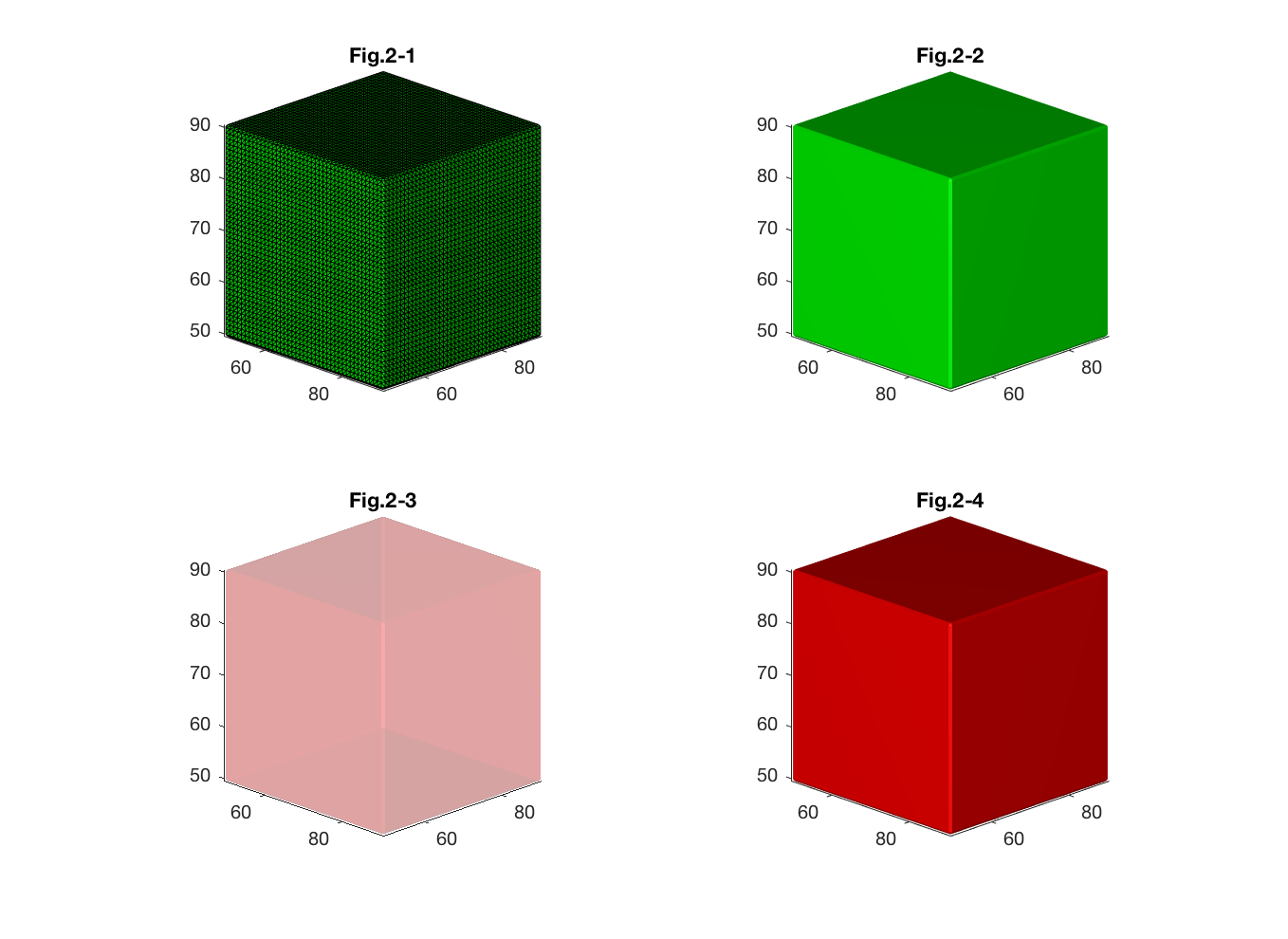

Instead of using one color for all faces/vertices of the surface, 'FaceVertexCData' property sets one color per face/vertex. It is an important property to visualize surface geometrical features.

In this example we specify a color for each vertex. Therefore, by setting 'FaceColor' property to 'flat, the color of the first vertex specified determines the face color (Fig. 3).

colorCode=myCubeSurface.vertices(:,3);   % Number of colors must equal number of vertices or faces
figure;
patch('Faces',myCubeSurface.faces,'Vertices',myCubeSurface.vertices,'FaceVertexCData',colorCode,'FaceColor','flat','EdgeColor','none');
view([45,20])
camlight(-10,10)
axis equal
title('Fig.3')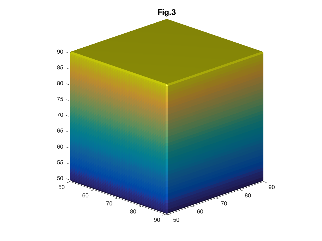

You can also set 'FaceColor' property to 'interp' which determine the face colors by using a bilinear interpolation of the values at each vertex (Fig. 4).

figure;
patch('Faces',myCubeSurface.faces,'Vertices',myCubeSurface.vertices,'FaceVertexCData',colorCode,'FaceColor','interp','EdgeColor','none');
% patch('Faces',myCubeSurface.faces,'Vertices',myCubeSurface.vertices,'FaceVertexCData',colorCode,'FaceColor','interp','EdgeColor','none','EdgeLightin','flat');
view([45,20])
camlight(-10,10)
axis equal
title('Fig.4')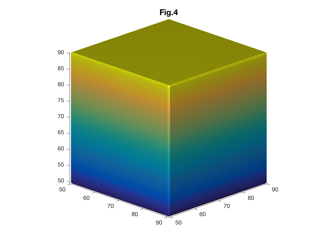

Predefined MATLAB colormaps can be used to color-code the surface. After color-coding the surface, it is useful to separately display a colorbar so that the meaning of each color can easily be understood. A colorbar can be displayed by using the funciton 'colorbar' or pushing the colorbar icon in the figure toolbar (Fig. 5).

% Set colormap to jet
colormap(jet)
colorbar
title('Fig.5')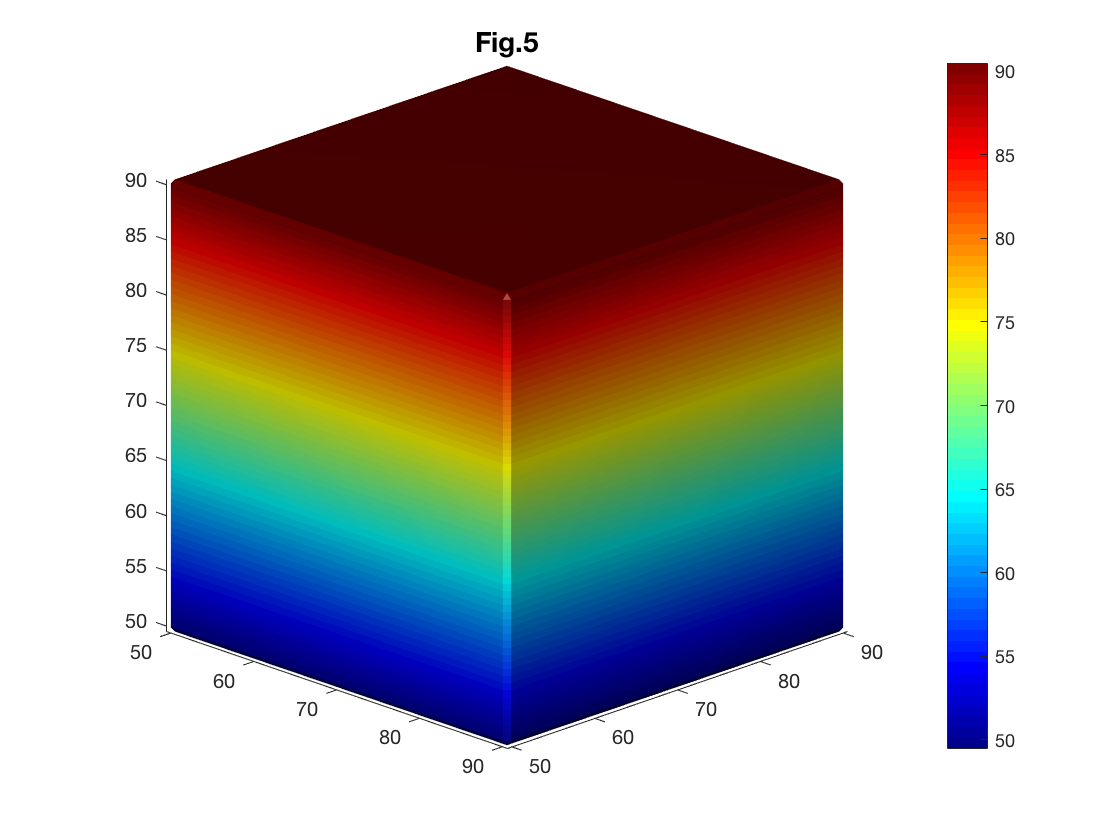

To save a created surface, the triangulated mesh can be converted to commonly used surface file formats such as Polygon File Format (.ply). The function tri_mesh_to_ply accepts a surface object and returns a PLY format structure.

% Convert triangulated mesh to Polygon File Format .ply
myCube_ply = tri_mesh_to_ply(myCubeSurface.vertices',myCubeSurface.faces');

The PLY structure can be saved outside MATLAB using the function 'ply_write'.

% Export surface file (.ply) to current directory
ply_write(myCube_ply,'myCube.ply');

Similarly the simulated volume can be saved as a nifti file for future use.

% Create Nifti (.nii) volume file
myCube_nii=make_nii(myCube);

% Save .nii file to current directory
save_nii(myCube_nii,'myCube.nii')

Challenge!

%%% Challenge 1: Making a cubiod shaped 3D volume and 3D surface.

% Part 1. 
% Using the worked example as a guide, write a script that creates a cuboid with 
% width and depth 80 and height 40 voxels in the center of a 100x100x100 frame 
% and assign it to a variable named MyCuboid.

% Part 2. 
% Extract myCuboid surface and assign it to myCuboidSurface variable.
% Visualise the cuboid using a color of your choice.

Challenge!

%%% Challenge 2

% Part 1: Plot the created cuboid again and color-code the width

% Part 2: Visualise the surface again with its width color coded and
% different surface transparency by using 'Alpha' in patch command
% Hint: search documentation for patch properties

% Part 3: Change the edges from The default color, black, to no edge displayed.
% Change the color distribution on each face to a smoother representation
% Hint: change patch properties EdgeColor and FaceColor

Challenge!

% Extension Challenge:
% Part 1: Make a cylinder with radius 50 and height 200 in 240x240x240 frame. 
% Part 2: Repeat challenge 2 using the cylinder created in pervious step.

Anatomical data

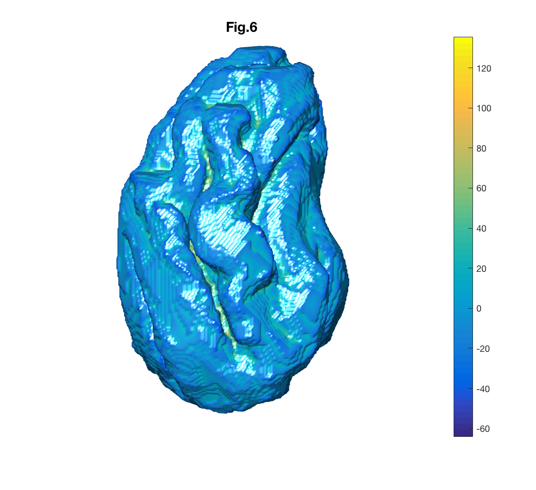
We can apply what we learned so far on anatomical data such as extracting and visualizing sheep brain surface from its volumetric binary mask, 'sheepBrain.nii'.

% Reading nifty file sheepBrain.nii then assigning it to variable sheepBrain_nii
sheepBrain_nii=load_nii('sheepBrain.nii');
% Extracting its surface and assigning it to sheepBrainSurface variable
sheepBrainSurface=isosurface(sheepBrain_nii.img);
load('sheepBrainCurvature')
% Visualising the brain surface and colorcode its curvature
figure
patch('Faces',sheepBrainSurface.faces,'Vertices',sheepBrainSurface.vertices,'FaceVertexCData',sheepBrainCurvature,'EdgeColor','none','FaceColor','interp','FaceLighting', 'gouraud');
view([-25,10])
camlight(-10,10)
axis equal
axis off
title('Fig.6')

Patch property 'FaceLighting' adjusts the light for object faces. To view curved anatomical surfaces 'gouraud' is used which calculates the light at the vertices and then linearly interpolate the light across the faces.

Another popular surface file format is '.stl'. MATLAB does not have an in-built function for reading .stl files but a function called 'stlread' is available to download from Mathworks website. (This function is provided in lesson repository.)

[femurSurface.faces,femurSurface.verices]=stlread('femurSurface.stl');
figure
patch('Faces',femurSurface.faces,'Vertices',femurSurface.vertices,'FaceColor','y',...
'EdgeColor', 'none');
camlight(-10,10)
axis equal
title('Fig.7')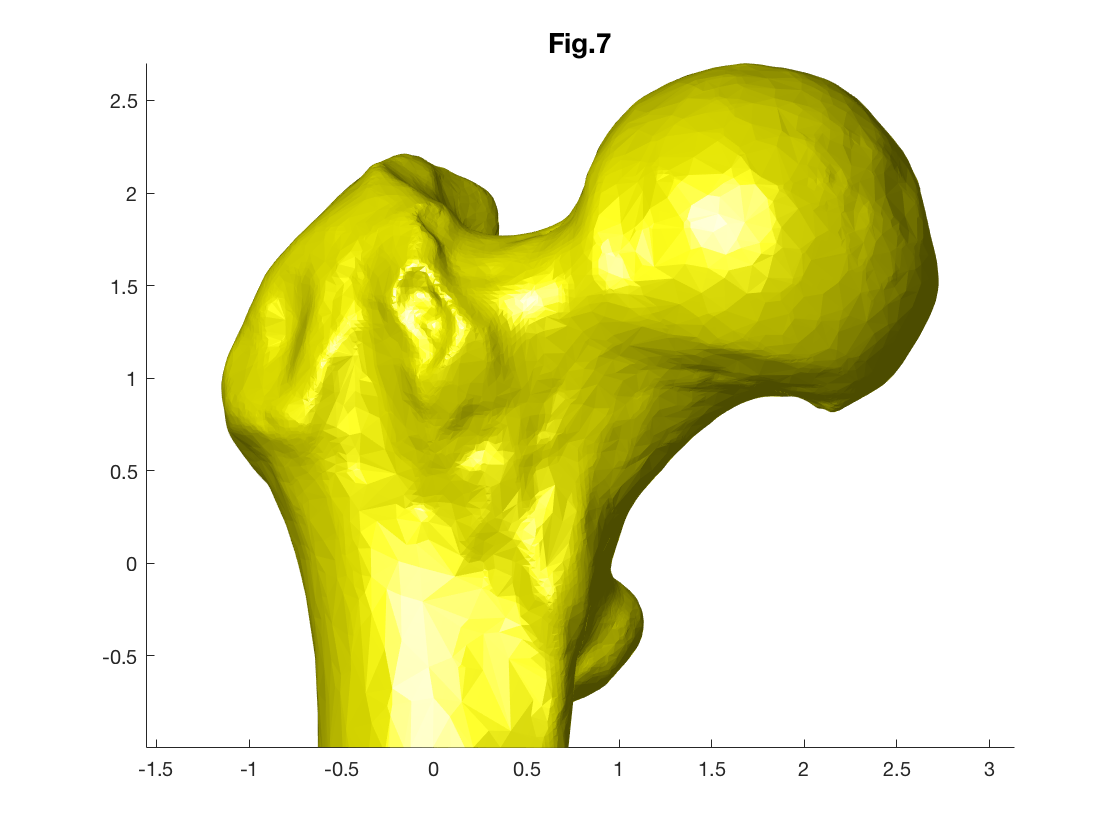

Similarly, Ply file format can be read into MATALB using the Mathworks function 'ply_read'.

[humanBrain_L_white.faces,humanBrain_L_white.vertices]=ply_read('humanBrain.L.white.ply','tri');
load('humanBrainCurvature_L_white');
figure;
patch('faces', humanBrain_L_white.faces', 'vertices', humanBrain_L_white.vertices','FaceVertexCData', humanBrainCurvature,'edgecolor','none','FaceColor','interp', 'FaceColor','interp','FaceLighting', 'gouraud','AmbientStrength', 0.9);view(-90,0);
camlight;
colormap('jet');
axis equal; axis off;
title('Fig.8')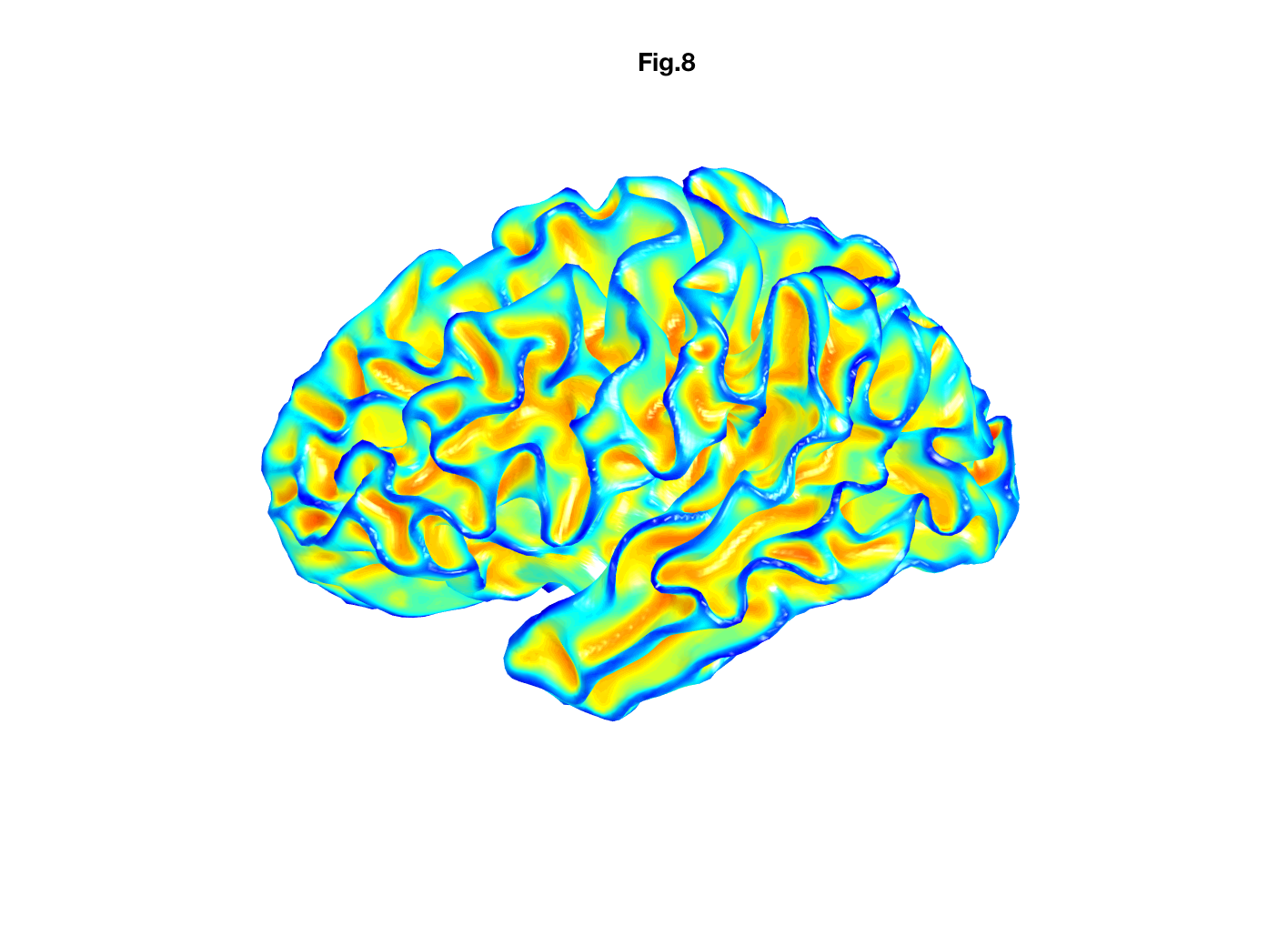

To illuminate the entire scene, Patch property ' AmbientStrength' is used.

The last file format that we introduce is GIfTI (.gii), the Geometery format under the NIfTI (.nii) format. It is a surface-file format complement to the NIfTI volume-file format. GIfTI is used in famous medical imaging software packages such as FreeSurfer, Caret and AFNI.

To read '.gii' surface data, a freely available MATLAB function 'gifti' is used.

addpath('gifti-1.6');
humanBrain_L_pial= gifti('humanBrain.L.pial.gii');
fcolor = [0.6 0.3 0.3];  
figure;
patch('faces', humanBrain_L_pial.faces, 'vertices', humanBrain_L_pial.vertices,'FaceColor', fcolor,'edgecolor','none', 'FaceLighting', 'gouraud','AmbientStrength', 0.9);view(-90,0);
camlight;
axis equal; axis off;
title('Fig.9')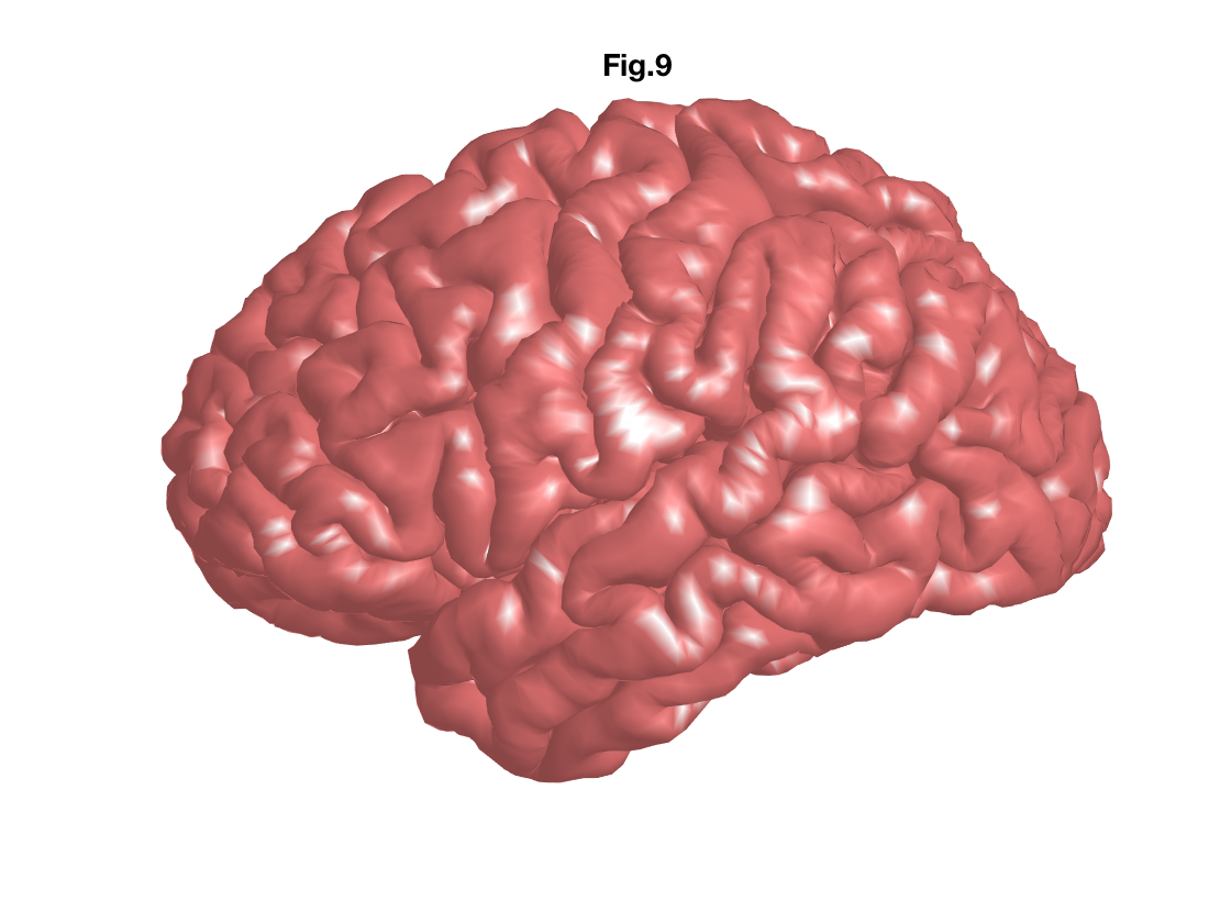

Challenge!

% Challenge3
% Part 1: Read human data humanBrain.L.pial.gii and humanBrain.R.pial.gii,
% Part 2: Visualise them both in one frame with your color of interest with
% some degree of transparancy,
% Part 3: Shine light on the object from different directions and try changeing the
% camera view,
% Part 4: Read human data humanBrain.L.white.ply and humanBrain.R.white.ply,
% Part 5: Visualise the white matter surfaces in the same frame that you presented the pial surfaces with their curvature colorcoded and with
% no transparancy.

Challenge!

% Extended challenge
% 
% Part 1: Read STL file humanBrain.stl and assign it to humanBrainSurface variable.
% Hint: use MATLAB function stlread.m
% Part 2: Transform the surface 50 voxels up.
% Part 3: Visualise the original and the transformed surfaces in one fram.
% Part 4: Convert the new surface to PLY file format.
% Part 5: Save the new ply file.
% Hint use tri_mesh_to_ply.m and ply_write.m functions

Acknowledgements

Sheep brain have been provided by the Animal MRI Laboratory at the Florey Institute of Neuroscience and Mental Health, A/ Prof. Leigh Johnston.
The Femur data and stlread function are downloaded from MathWorks (http://au.mathworks.com/matlabcentral/fileexchange/22409-stl-file-reader ) and provided by Eric Jonson.
Human brains visualised in this section are coming from Connectome DB and Connectome Workbench, developed under the auspices of the Human Connectome Project at Washington University in St. Louis and associated consortium institutions (http://www.humanconnectome.org/).

3D Structural Modelling

3D Structural Modeling

Learning Objectives

Simulated data

Anatomical data

Acknowledgements

results matching ""

No results matching ""