MRI Data Visualization

Author: Syeda Warda Taqdees

Contributor/s: Dr. Christina Tuke Flanders, Asif Iqbal, Akhil

Learning Objectives

After completing this lesson, students should be able to

• Create a montage of MRI slice data.
• Display MRI slice data sequentially using 'imagesc' function.
• Create grid view of MRI slice data using 'subplot'.
• Index MRI slice data to view in axial, coronal and sagittal directions.
• Take Affine transform of coronal and sagittal slices for improving image quality.
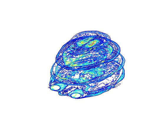
• Display a stack of slice contours with suitable colormaps.

MRI image volume-data is an 'MxNxK' dimensional dataset, consisting of 'K' 2D images, called 'slices', of 'MxN' dimensions. Each slice in an MRI dataset has same orientation ('axial', 'coronal' or 'sagittal') depending on scanning parameters.

MRI image dataset can be visualized in MATLAB in different ways. In this section, we will discuss the commonly used methods for visualizing MRI data.

Montage

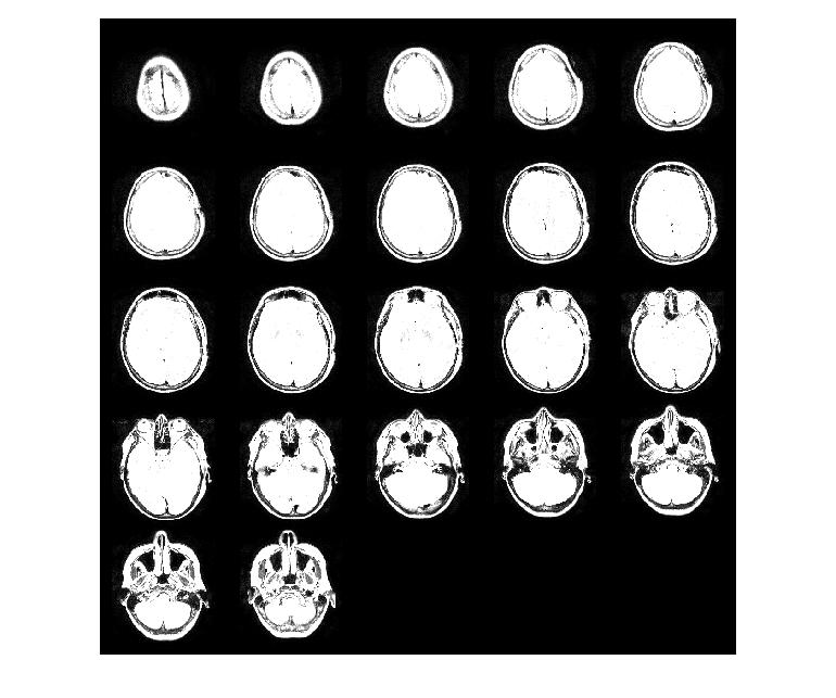
A montage is created by putting together image slices into a single image.

MATLAB function 'montage' accepts an MxNx1xK image dataset and displays multiple image frames as a montage. 'reshape()' is used to resize MRI image dataset for creating montage.

% MRI images can be displayed as a montage
% Image dimensions must be MxNx1xk
montageImg = reshape(mriImage,[512 512 1 22]);

% Montage colormap
montageCMap = gray(128);

% Displaying Montage Image
montage(montageImg, montageCMap);

Challenge!

% Challenge 1
% Download an MRI dataset of your choice. 
% Create Montage of the images with multiple intensity ranges
% Extension: Create montage of every other image in the dataset

Imshow()

Sequential Display

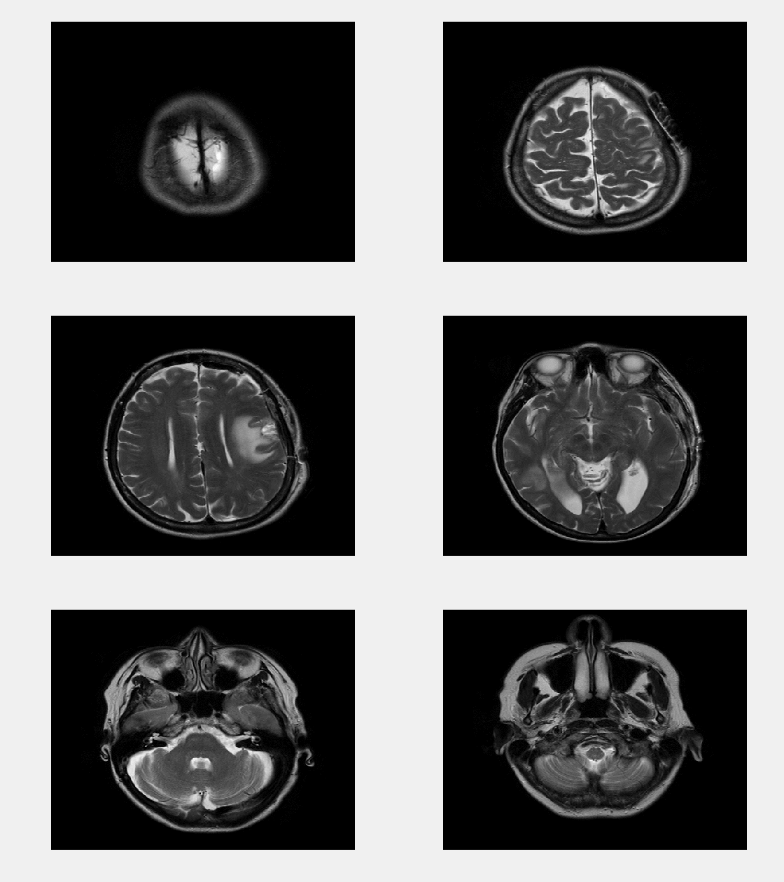
In last section, we learned that 'imagesc' is a convenient way for displaying a single image slice. 'imagesc' can be paired with 'pause' command in a loop to display all image slice sequentially for viewing image slices sequentially.

% imagesc can be used in a loop to display a range of slices sequentially
figure;

for iImg = 1:22
    imagesc(mriImage(:,:,iImg));
    axis off; colormap gray
    hold on;
    
    % pause(n) slows down image display
    pause(0.3)   
end

Slice Grid

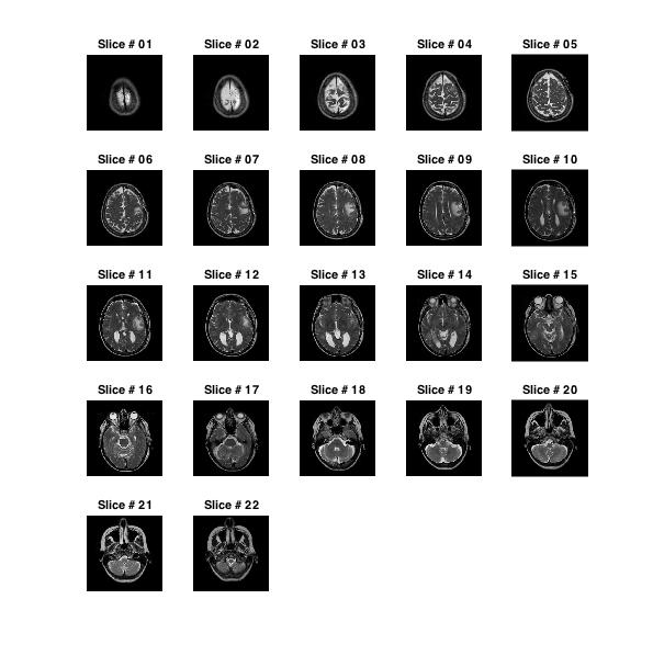
Another way to visualize MRI data is to used 'subplot' for displaying a gird of slices. Unlike montage, that creates a single image from all slices, a slice grid displays each slice in a separate figure. This allows us to change display properties of each slice individually.

% subplot can be used to display montage-like image slice.  
figure;
for iImg = 1:22
    subplot(5,5,iImg)
    imagesc(mriImage(:,:,iImg));
    
    % Setting display properties
    colormap gray
    axis image;
    axis off; colorbar
    title(sprintf('Slice # %02d',iImg))      
end

Challenge!

% Challenge 2

% Create montage of your downloaded MRI images using subplot.
% Assign different colormaps to different slices e.g. slice#1 gray, slice#2
% jet, slice#3 gray and so on
% Display colorbar for each slice.
% Extension: Flip slices along y-direction, Flip slices along x-direction
% set cLim property of slice images so that each colorbar has same range.

Coronal and Sagittal Slice Extraction

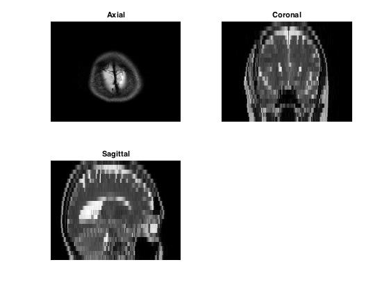
In this workshop, we are working on a 3D MRI dataset consisting of axial slices. We can extract sagittal and coronal slices from this axial data by indexing.

% MRI image array can be indexed to display slices in axial, coronal or
% sagittal view

figure
%Displaying axial slice
subplot(2,2,1);
imagesc(mriImage(:,:,1));
colormap gray; axis off;
title('Axial')

%Displaying coronal slice
subplot(2,2,2);
corSlice = squeeze(mriImage(200,:,:));
imagesc(corSlice);
colormap gray; axis off
view(90,90)
title ('Coronal')

% Displaying sagittal slice
subplot(2,2,3);
sagSlice = squeeze(mriImage(:,200,:));
imagesc(sagSlice);
colormap gray; axis off;
view(90,90);
title('Sagittal')

Challenge!

% Challenge 3
% Diplay axial, sagittal and coronal slices of your downloaded MRI data.
% Set axis image and observe changes in coronal and axial slices.
% Extension: Loop through all sagittal slices for axial-slice# 10 and coronal-slice#
% 300.

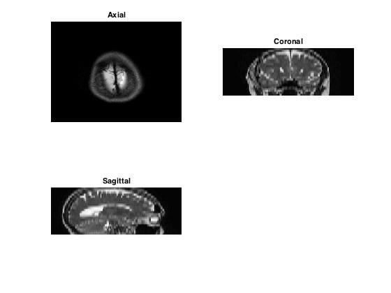
Notice that in the previous section, the dimensions of coronal and sagittal slices are 512x22. Thus, the images created for these views have very low resolution and they appear pixelated.

One way to improve sagittal and coronal slice resolution is by scaling and resampling image data along these orientations. This is achieved by taking an affine transform. The function maketform accepts a 3x2 transform matrix and returns a spatial transform structure. Resampling properties are defined in a structure returned by 'makeresampler'. More information on affine transform can be found here.

Finally, the slice is spatially transformed using 'imtransform'.

% To improve image quality of coronal and sagittal views
% Affine transform, followed by interpolation is carried out. 

% Defining affine transform
T0 = maketform('affine',[2 0; 0 .23; 0 0]);

% Creating resampling structure
R2 = makeresampler({'cubic','nearest'},'fill');

figure;
%Displaying axial slice
subplot(2,2,1);
imagesc(mriImage(:,:,1));
axis off;
colormap gray;
title('Axial')

%Displaying coronal slice
subplot(2,2,2);
corSlice = squeeze(mriImage(200,:,:));

% taking image transform
corSliceT = imtransform(corSlice,T0,R2);

%Displaying image
imagesc(corSliceT);
colormap gray; 
axis image; axis off
view(90,90)
title ('Coronal')

% Displaying sagittal slice
subplot(2,2,3);
sagSlice = squeeze(mriImage(:,200,:));

% taking image transform
sagSliceT = imtransform(sagSlice,T0,R2);

% Displaying image
imagesc(sagSliceT);
colormap gray; 
axis image; axis off
view(90,90)
title('Sagittal')

Challenge!

% Challenge 4 
% Try different values for affine transform(scaling and rotation) matrix. 
% Open documentation for makeresampler and change properties of interpolation object.
% Apply it on coronal and axial slices of your choice and observe effects
% of these changes. 

Advanced Visualization Techniques

Viewing NIfTI files

In previous section, we created '.nii' file for our data. NIfTI files can be viewed in MATLAB using 'view_nii' function provided in the course repository.

% view_nii is a useful function for visualizing NIfTI files
view_nii(mriImgNifti);

Challenge!

% Challenge 5
% View NIfTI file of 'myImg' created in Part 1.

3D Contour Slices

Each slice in image dataset is a 2D object and when stacked together create a 3D volume data object. By using 'contourslice' we can create a 3D object consisting of slice contours which can then be viewed in any orientation.

% 'contourslice' can be used to display stack of slice contours

figure
cm = gray(50);
cHandle = contourslice(mriImage,[],[],[1 5 15],8);
colormap(cm)
set(cHandle,'FaceColor','interp')